Is your neighborhood fat?

Obesity is a serious health condition that jeopardizes an individual’s well being. Being obese means having a body mass index greater (BMI) greater than 30. This increases the risk of developing a plethora of debilitating health conditions such as coronary heart disease, diabetes, depression, stroke, and even cancer. We often hear in the news about the obesity epidemic in America. According to the CDC as many as 35 percent of Americans are considered obese. This monumental figure sparked my interest in investigating why obesity is so prevalent within our population. Thus, I looked online for data to see what is causing this obesity epidemic. I found 6 data sets from the Community Status and Health Indicators (CHSI) database that described the demographics, social behaviors, causes of deaths, preventive services use, environmental statistics, and importance of health by county. After exploring the data, I saw that the obesity rate for around 30% of the counties were missing. Therefore, I decided to predict whether these missing counties were above or below the median obesity rate.

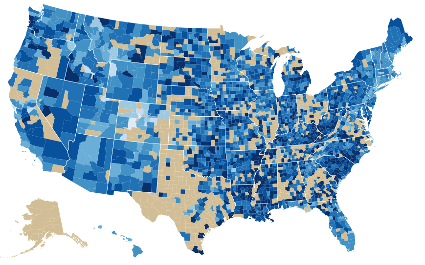
The graph below was made using d3.js and visualizes the obesity rate by county. The darker blue means that there is a higher obesity rate. The gray means that the obesity rate is missing for these counties.

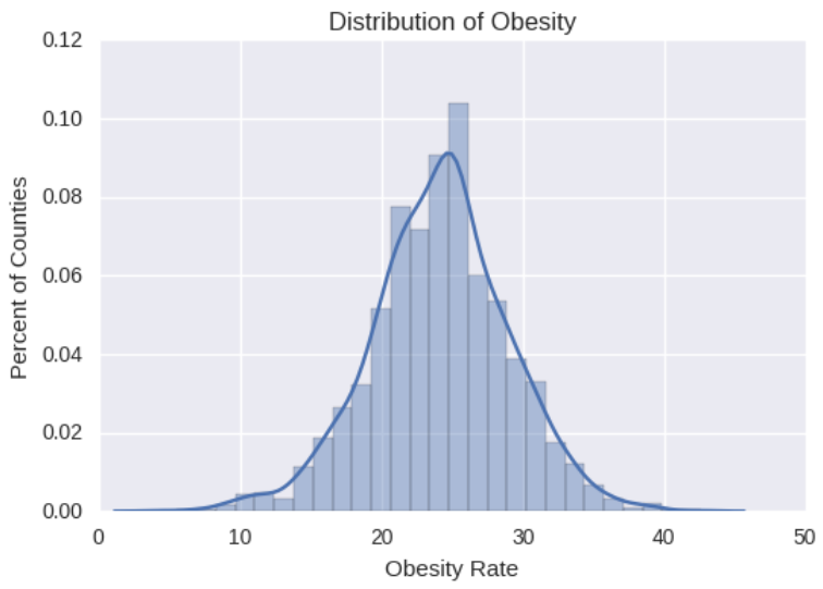
The chart below shows the distribution of obesity rates throughout the United States. The mean and median are around 24%.

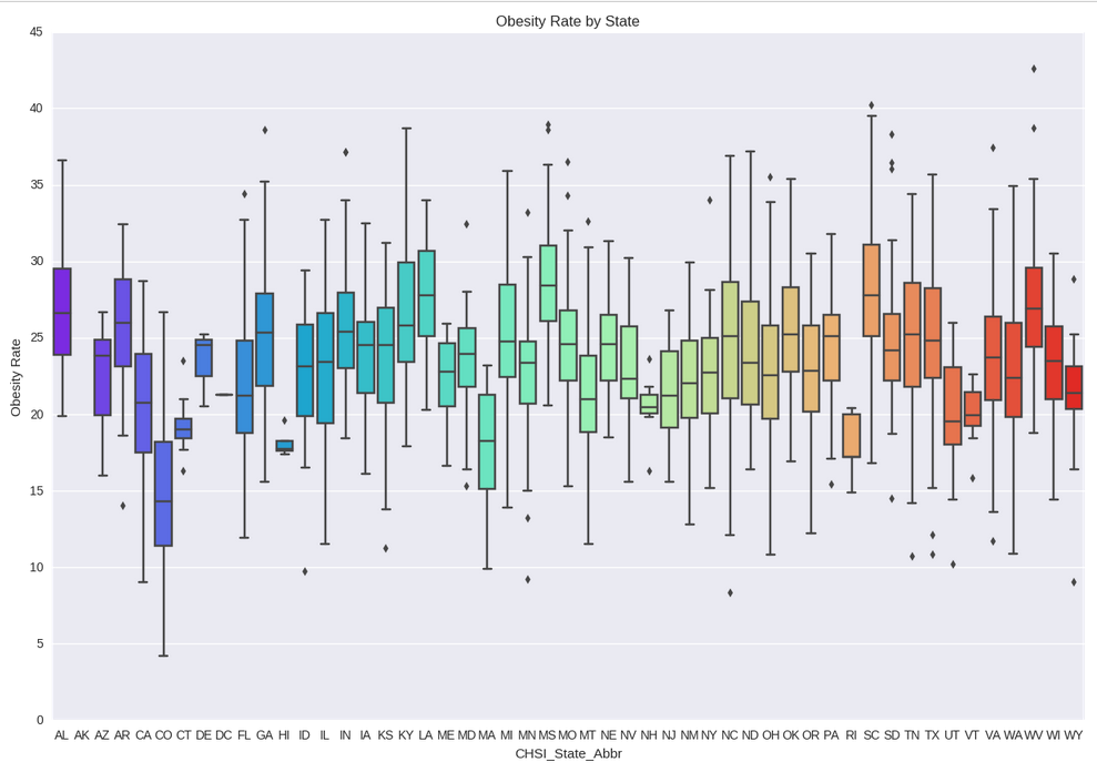
Another visualization of the obesity rates by state.

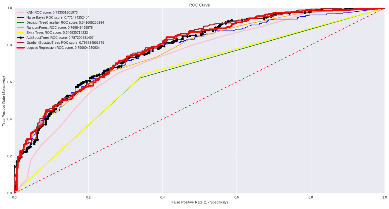
Combining all the data sets gave me around 500 features. There are only 3142 counties so I had to reduce the dimensionality of the data. I did so by adding random noise to the data and running a random forest model several times to determine the most important features that affect obesity rates. My next step was experimenting with several classification algorithms with the 20 features my random forest model selected. The graph below shows the ROC score of all the different models that were used. We can see that Ada Boosted Trees, Gradient Boosted Trees, and Logistic Regression all had a similar performance. For the sake of interpetation, I decided to further my analysis with Logistic Regression.

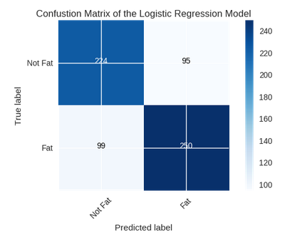
The chart below shows the confusion matrix for the logistic regression model. We can see that it performed generally well with both classes. The precision and recall scores were both 0.71.

The features that gave a higher probability of having high obesity rates were counties with high rates of:

1. No exercise
2. Diabetes
3. Primary care physician visits
4. Poverty
5. Asian population
6. Toxic chemicals
7. Recent drug use
8. Females with heart disease
9. Population under 19 years old
10. White population

The features that gave a lower probability of having high obesity rates were counties with high rates of:

1. Few fruits and vegetables consumption
2. Black population
3. Population between ages 19-64
4. Dentist visits
5. Depression

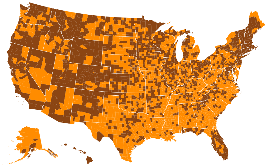
These results can imply that educating people younger than 19 years about diet and exercise is an effective way of fighting obesity. In addition, race and culture has an affect on obesity. The graph below shows the predictions of the counties with the missing data along with the data from the training set. Orange means that the county has an obesity rate higher than the median and brown means that the county has an obesity rate lower than the median.